Redundancy and Efficiency in Neural Networks

Did you know we only use 10% of our brains? Well, if you did, you'll be happy to learn that it is entirely false.

But imagine if the myth were true. You'd be feeding this huge brain with calories, but you'd get only a tiny bit of benefit in return. This might not be true in brains, but it's very common in machine learning models. You feed it time and money, even though you often aren't using the whole thing.

The concept of neuron pruning, much like pruning in agriculture, is to remove the parts of the model that aren't contributing to how well it works. We remove brain cells, or neurons, to reduce the model's size without a significant drop in the quality of the fruits it bears. Unlike agriculture, though, in machine learning we can test the pruned model and put neurons back if needed, so we can optimise the model to make it as efficient as possible.

Nodes, Activation, Features, and Targets

Neurons are often referred to as nodes in machine learning. The nodes perform calculations in a sequence: each node receives input, performs a small calculation, and passes the output to the next node. At the start of this sequence, we input features, like the information that is passed on to your brain: your eyes see something yellow and round, and your eyes pass on the features shape=round and colour=yellow. At the end of the sequence, it outputs a prediction: for example, you might be looking at the sun.

For now, we'll ignore the nodes in the middle of the sequence and focus on the nodes that receive input features and return the targets we're trying to predict. This will make it easier to see where redundancies come from, and to understand when we start looking at redundancies in the middle of the sequence in future posts.

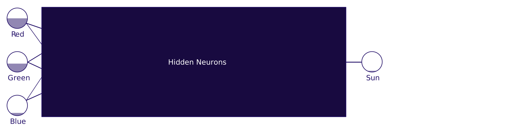
Realistically, the input feature that tells us we're looking at something yellow will actually tell us how yellow the thing we are looking at is. Considering how an eye works, it is more likely to be three different features, something like red: 5, green: 4, blue: 1. From this input we can say with a high level of confidence that we're looking at yellow, but we can never be certain we're looking at the sun; in fact there are many things it could be. The output is a prediction, so we might have an output like sun: 0.2. These numbers are called the activation values, think of them like a dimmer switch for a light bulb. The neurons in your brain activate to different intensities just like a dimmer switch, and so do the nodes in our neural network.

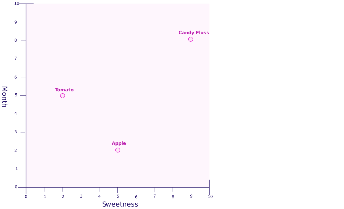
Let's start with a very simple example: your brain has a specific node that lights up when you taste sweet things. The sweeter the food, the stronger the activation value:

• Tomato: 2 sweetness
• Apple: 5 sweetness
• Candy floss: 9 sweetness

It can be useful to be able to visualise our activations in case we see patterns. We could plot the activations for the sweetness feature on a single "sweetness" axis to visualise it.

Then we can add a second feature to our neural network to start looking for patterns. Let's also log the time of year we ate the food. We now have a sweetness feature and a month feature. We can visualise how the activation values for three food items like this:

Features With Low Predictive Relevance

At first, you might think the above plot doesn't look very useful, but it really depends on our target. Remember, the target is the prediction we're trying to get out of our neural network. If our target is to predict the outside temperature when we're eating, then the month feature may be more useful for our neural network. When I eat food in June, it's warmer outside than when I eat food in December. However, if the goal is to predict how satisfied we are after eating or how tasty we find the food, then the sweetness feature may be more useful.

For now, let's consider that we train two different neural networks. We taste 1000 foods, and for one network we log the features 'month', 'sweetness' and the target 'outside temperature', and for the other we log the features 'month', 'sweetness' and the target 'tastiness'. We can then train these two networks (we won't discuss how we train networks in this post) so they can make predictions for us in the future.

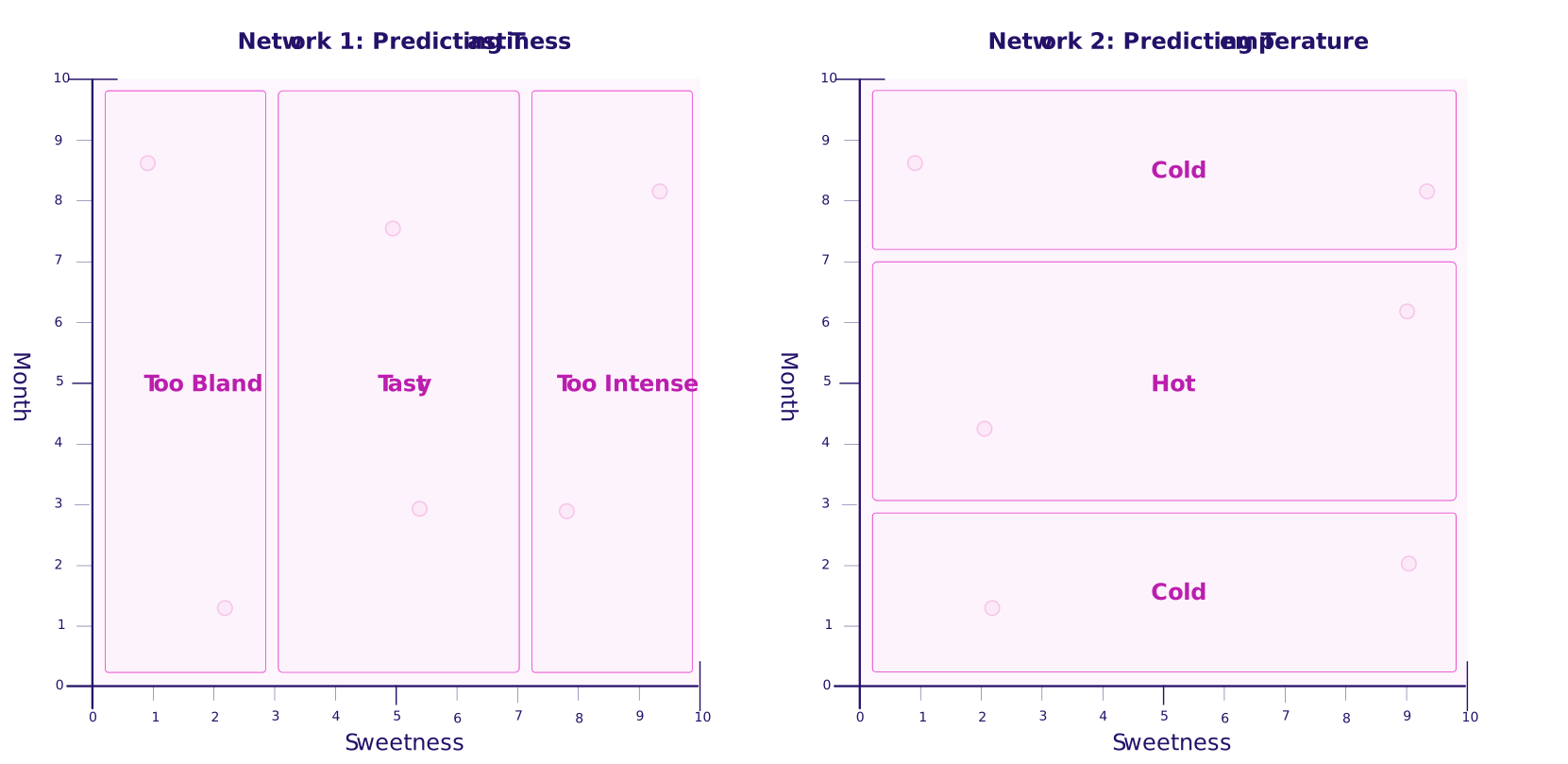
After training, one network has identified a pattern between the month and how hot it is outside, while the other has identified a pattern between sweetness and how tasty the food is. Now, if you consider eating something of average sweetness in June, you can put the data into one neural network to identify that it has a high probability of being tasty and another neural network to predict that it has a high probability of being hot outside.

It should be clear that each of these neural networks contains an entirely redundant feature. If we want to predict the outside temperature, the sweetness feature has low predictive relevance; if we want to know how tasty some food is, the month feature has low predictive relevance.

From here we can try removing a feature from each of these two neural networks (month from the network that predicts tastiness and sweetness from the neural network that predicts temperature) and retrain and test the networks. If the output (or accuracy on our test data) is essentially unchanged, we can confirm the feature was redundant for that task.

However, if we do see a change (maybe people eat more ice cream on hot days and tastier savoury food at Christmas), then we will have a decision to make between the loss in accuracy and the reduction in cost of the neural network. I'll refer to this in future posts as the cost–accuracy trade-off.

Summary

Neural networks can end up larger than they need to be, and visualising and testing neurons or features helps reveal which ones actually matter. That understanding lets us prune with intent, deciding whether to trade a small amount of accuracy for meaningful savings in cost and runtime.

Everything in this post should be intuitive, but once we consider neural networks with more than two features, or look at the hidden neurons that appear in the middle of the sequence in our neural network, it can get much harder to visualise and comprehend. We'll build on this concept in the next few posts.

Glossary

• Neural Network: a computer program that makes predictions.
• Node/Neuron: a single unit of a neural network that receives an input, performs a small calculation, and passes the output to the next unit.
• Activation: the output value of a single neuron after it's completed its calculation.
• Feature/Input Variable: the initial values you put into a neural network, such as sweetness or red.
• Target/Output Variable: the quality you're trying to predict, such as tastiness or temperature.
• Predictive relevance: how much a feature or a node helps the network make an accurate prediction.
• Redundancy: a feature or part of the network that does not add meaningful information.
• Neuron Pruning: the process of removing and testing potentially redundant parts of a neural network.
• Cost–accuracy trade-off: deciding if a reduction in cost is worth a reduction in efficiency.